- Published on
Exponential Approximation with Least Squares in Python
- Authors

- Name
- Daisuke Kobayashi
- https://twitter.com
Recently I have occasionally needed to do simple data analysis at work. The task itself is straightforward: fit a curve to measured data and obtain an approximate formula.
You can do that in Excel by plotting the data and asking it to add a trendline formula, but creating a graph every time is tedious. Once you start thinking about evaluating the fitted formula automatically, it becomes hard not to want to script the whole process.
When that happens, I usually write a Python script.
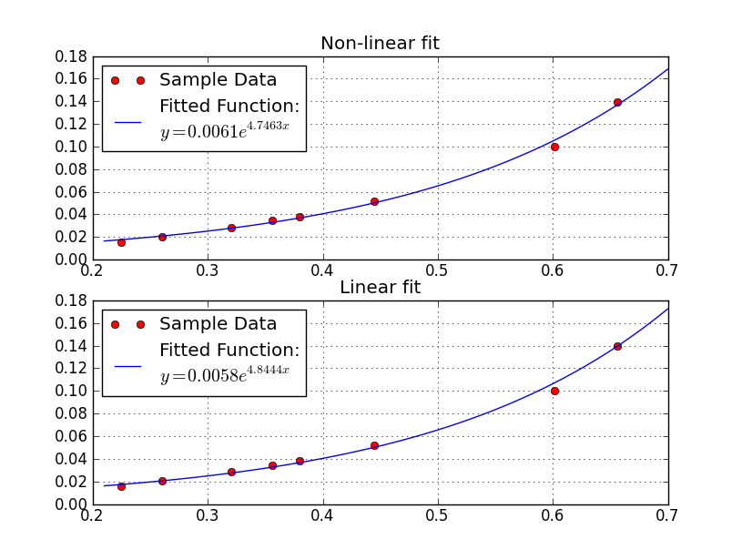
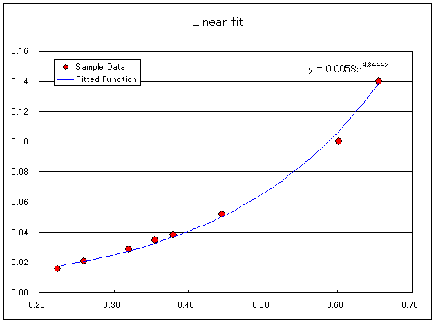
This time I wrote a script that uses least squares in SciPy to obtain an approximate formula, but I ran into a problem: the numbers were slightly different from the equation produced by Excel. I got stuck on that for about half a day, so I am leaving a note here.
The conclusion is simple: the problem was applying least squares directly to the exponential function.
Suppose the function we want to fit is y = a * exp(b * x). Then the problem is to find (a, b) from measured data (**x**, **y**) so that the sum of squared errors of y = a * exp(b * x) is minimized.
You can solve that problem directly, but Excel seems to take the logarithm of both sides and then fit the transformed equation below instead.
log(y) = log( a * exp( b * x ) )
log(y) = ( log(a) + b * x )
When I compared fitting the original form and the transformed form in Python against Excel, the log-transformed version matched the equation from Excel.
Here is the Python code I used.
#! /usr/bin/env python
# -*- coding: utf-8 -*-

import numpy
import scipy.optimize
import matplotlib.pyplot as plt

def fit_exp(parameter, x, y):
    a = parameter[0]
    b = parameter[1]
    residual = y - (a * numpy.exp(b * x))
    return residual

def fit_exp_linear(parameter, x, y):
    a = parameter[0]
    b = parameter[1]
    residual = numpy.log(y) - (numpy.log(a) + b * x)
    return residual

def exp_string(a, b):
    return "$y = %0.4f e^{ %0.4f x}$" % (a, b)

if __name__ == "__main__":

    x = numpy.array([6.559112404564946264e-01,
                     6.013845740818111185e-01,
                     4.449591514877473397e-01,
                     3.557250387126167923e-01,
                     3.798882550532960423e-01,
                     3.206955701106445344e-01,
                     2.600880460776140990e-01,
                     2.245379618606005157e-01])

    y = numpy.array([1.397354195522357567e-01,
                     1.001406990711011247e-01,
                     5.173231204524778720e-02,
                     3.445520251689743879e-02,
                     3.801366557283047953e-02,
                     2.856782588754304408e-02,
                     2.036328213585812327e-02,
                     1.566228252276009869e-02])

    parameter0 = [1, 1]

    r1 = scipy.optimize.leastsq(fit_exp, parameter0, args=(x, y))
    r2 = scipy.optimize.leastsq(fit_exp_linear, parameter0, args=(x, y))

    model_func = lambda a, b, x: a * numpy.exp(b * x)

    fig = plt.figure()

    ax1 = fig.add_subplot(2, 1, 1)
    ax2 = fig.add_subplot(2, 1, 2)

    ax1.plot(x, y, "ro")
    ax2.plot(x, y, "ro")

    xx = numpy.arange(0.7, 0.2, -0.01)

    ax1.plot(xx, model_func(r1[0][0], r1[0][1], xx))
    ax2.plot(xx, model_func(r2[0][0], r2[0][1], xx))

    ax1.legend(("Sample Data", "Fitted Function:\n" + exp_string(r1[0][0], r1[0][1])),
                "upper left")
    ax2.legend(("Sample Data", "Fitted Function:\n" + exp_string(r2[0][0], r2[0][1])),
                "upper left")

    ax1.set_title("Non-linear fit")
    ax2.set_title("Linear fit")

    ax1.grid(True)
    ax2.grid(True)

    plt.show()
It had also been a while since I last had to think about logarithms, and I realized I had forgotten more of the math than I expected. I should probably study mathematics again.
Reference: