Bayesian Linear Regression in Python

Following the least-squares method from the previous post, this time I will do exponential approximation with Bayesian linear regression.

There is a lot of theory behind it, but the final form only requires a small modification to the least-squares approach.

Bayesian linear regression has two parameters, and by adjusting them you can control the degree of fitting and prevent overfitting.

#! /usr/bin/env python
# -*- coding: utf-8 -*-

import numpy
import matplotlib.pyplot as plt


def least_squares_regression(X, t, phi):

    PHI = numpy.array([phi(x) for x in X])
    w = numpy.linalg.solve(numpy.dot(PHI.T, PHI), numpy.dot(PHI.T, t))

    return w


def bayesian_linear_regression(X, t, phi, alpha = 0.1, beta = 10.0):

    PHI = numpy.array([phi(x) for x in X])
    Sigma_N = numpy.linalg.inv(alpha * numpy.identity(PHI.shape[1]) + beta *
            numpy.dot(PHI.T, PHI))
    mu_N = beta * numpy.dot(Sigma_N, numpy.dot(PHI.T, t))

    return mu_N


def exp_string(a, b):
    return "$y = %0.8f e^{ %0.8f x}$" % (a, b)


if __name__ == '__main__':

    X = numpy.array([6.559112404564946264e-01,
                     6.013845740818111185e-01,
                     4.449591514877473397e-01,
                     3.557250387126167923e-01,
                     3.798882550532960423e-01,
                     3.206955701106445344e-01,
                     2.600880460776140990e-01,
                     2.245379618606005157e-01])

    t = numpy.array([1.397354195522357567e-01,
                     1.001406990711011247e-01,
                     5.173231204524778720e-02,
                     3.445520251689743879e-02,
                     3.801366557283047953e-02,
                     2.856782588754304408e-02,
                     2.036328213585812327e-02,
                     1.566228252276009869e-02])

    phi = lambda x: [1, x]

    w = least_squares_regression(X, numpy.log(t), phi)
    mu_N = bayesian_linear_regression(X, numpy.log(t), phi)

    lsq_a = numpy.exp(w[0])
    lsq_b = w[1]

    blr_a = numpy.exp(mu_N[0])
    blr_b = mu_N[1]

    fig = plt.figure()
    ax = fig.add_subplot(1, 1, 1)

    xlist = numpy.arange(0, 1.01, 0.01)
    ax.plot(X, t, "ko", ms=7)
    ax.plot(xlist, lsq_a * numpy.exp(lsq_b * xlist), "b-", lw=2)
    ax.plot(xlist, blr_a * numpy.exp(blr_b * xlist), "r-", lw=2)

    ax.legend(("Data",
               "Least squares: " + exp_string(lsq_a, lsq_b),
               "Bayesian linear: " + exp_string(blr_a, blr_b)),
               loc="upper left", shadow=True, fancybox=True)

    plt.show()

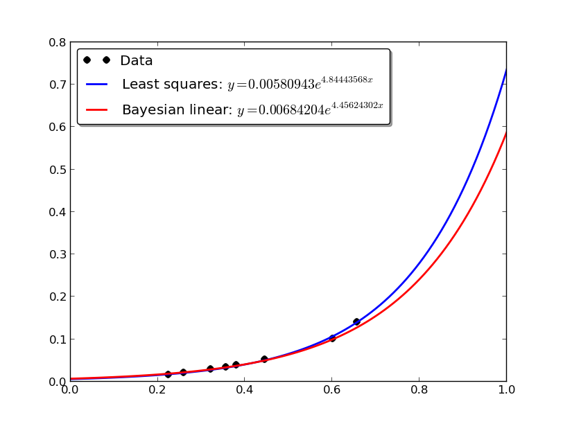
If you plot the graph, it looks like the figure below. Overall the number of data points is small, but if you look closely, Bayesian linear regression fits less aggressively where the x values are larger. Because the data is sparse there, Bayesian linear regression effectively treats those values as less reliable and prevents overfitting.

Reference:

http://gihyo.jp/dev/serial/01/machine-learning/0014