Python でベイズ線形回帰

前回の最小二乗法に続き，ベイズ線形回帰で指数近似を行います．

理論的にはいろいろありますが，最終的な形は最小二乗法をちょっと変形するだけです．

ベイズ線形回帰の場合には，パラメータが 2 つあり 2 種を調整することでフィッティングの度合いを調整し，過学習を防ぐことができます．

#! /usr/bin/env python
# -*- coding: utf-8 -*-

import numpy
import matplotlib.pyplot as plt


def least_squares_regression(X, t, phi):

    PHI = numpy.array([phi(x) for x in X])
    w = numpy.linalg.solve(numpy.dot(PHI.T, PHI), numpy.dot(PHI.T, t))

    return w


def bayesian_linear_regression(X, t, phi, alpha = 0.1, beta = 10.0):

    PHI = numpy.array([phi(x) for x in X])
    Sigma_N = numpy.linalg.inv(alpha * numpy.identity(PHI.shape[1]) + beta *
            numpy.dot(PHI.T, PHI))
    mu_N = beta * numpy.dot(Sigma_N, numpy.dot(PHI.T, t))

    return mu_N


def exp_string(a, b):
    return "$y = %0.8f e^{ %0.8f x}$" % (a, b)


if __name__ == '__main__':

    X = numpy.array([6.559112404564946264e-01,
                     6.013845740818111185e-01,
                     4.449591514877473397e-01,
                     3.557250387126167923e-01,
                     3.798882550532960423e-01,
                     3.206955701106445344e-01,
                     2.600880460776140990e-01,
                     2.245379618606005157e-01])

    t = numpy.array([1.397354195522357567e-01,
                     1.001406990711011247e-01,
                     5.173231204524778720e-02,
                     3.445520251689743879e-02,
                     3.801366557283047953e-02,
                     2.856782588754304408e-02,
                     2.036328213585812327e-02,
                     1.566228252276009869e-02])

    phi = lambda x: [1, x]

    w = least_squares_regression(X, numpy.log(t), phi)
    mu_N = bayesian_linear_regression(X, numpy.log(t), phi)

    lsq_a = numpy.exp(w[0])
    lsq_b = w[1]

    blr_a = numpy.exp(mu_N[0])
    blr_b = mu_N[1]

    fig = plt.figure()
    ax = fig.add_subplot(1, 1, 1)

    xlist = numpy.arange(0, 1.01, 0.01)
    ax.plot(X, t, "ko", ms=7)
    ax.plot(xlist, lsq_a * numpy.exp(lsq_b * xlist), "b-", lw=2)
    ax.plot(xlist, blr_a * numpy.exp(blr_b * xlist), "r-", lw=2)

    ax.legend(("Data",
               "Least squares: " + exp_string(lsq_a, lsq_b),
               "Bayesian linear: " + exp_string(blr_a, blr_b)),
               loc="upper left", shadow=True, fancybox=True)

    plt.show()

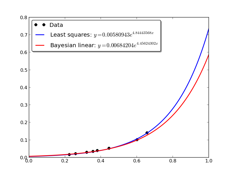
グラフを表示すると下記のようになります．全体的にデータ数が少ないですが，グラフを見ると，ベイズ線形回帰の方は x の値が大きい方でのフィッティング度合いが弱くなっています．データ数が疎であるため，ベイズ線形回帰では値を外れ値と見なし，過学習を防いでます．

参考:

http://gihyo.jp/dev/serial/01/machine-learning/0014